Waterfall Chart using Power Query

How to create a Waterfall Chart using Power Query?

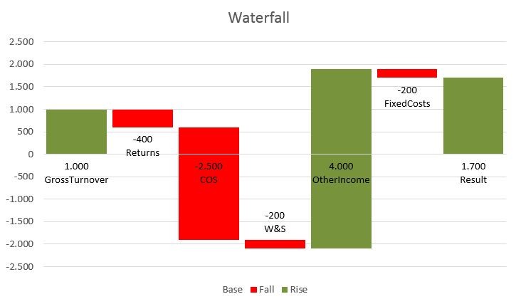
Target is a chart like above: Starting point, several movements & then an ending sum. Every movement starts at the end of the previous movement, upsides in green colour, downsides in red.

The source data for this kind of charts are normally missing the last line like this example with a P&L:

So this makes it always a bit clumsy to integrate in an automatically refreshing reporting package, especially if the number of lines/bars to report is dynamic.

So here comes the Power Query solution: Fully automatic & dynamic – calculation & charting.

Simply update your source data (Table: “Sourcedata”) & the rest will be done automatically. In this simple example the order of the Sourcedata-table will be kept in the chart.

Refresh the query or check “Data – refresh all” – done.

You can use this as it is – just prepare your table accordingly (fill in your numbers manually, create links or a power query to your source data… however), no need to adjust the query or even have a look at it.

Waterfall

 

But if you’re interested in how this works, just read on 🙂

let Source = Excel.CurrentWorkbook(){[Name="Sourcedata"]}[Content],
This step imports the source data: A table called “Sourcedata”

AppendLastRow = Table.Combine({Source,WaterfallEnd}),
Here we’re appending the ending row, which we’ve simply pushed into PQ (Query WaterfallEnd)

AddIndex = Table.AddIndexColumn(AppendLastRow, "Index", 0, 1),
This step adds a standard-Index-column that will give us the row number for the cumulation.

Cum = Table.AddColumn(AddIndex, "Cum", each List.Sum(List.FirstN(AppendLastRow[Amount],[Index]+1))),
As for the cumulation we want to add up all amounts up to the current row. This is how we address the column with the amounts (reading the nested formular from inside out):

• AppendLastRow[Amount]. Reading: In the brackets stands the name of the column, before the name of the table. So we’re reaching out for the table from a previous step (AppendLastRow) and grabbing the column “Amount”.
• But we don’t want to sum up the whole column, just the rows up to the current index value. Therefore we’re using “List.FirstN(AppendLastRow[Amount],[Index])”. Having our freshly retrieved column as the first part of the expression & [Index] as the number of first rows to keep (we need to add 1, because our index started at 0).
• Last step is to add this, using “List.Sum” on all of it.

 CumPrev = Table.AddColumn(Cum, "CumPrev", each try(Cum[Cum]{[Index]-1}) otherwise null),
For our “Fall” column we need the Cum of the previous row. As we’ve learned in the previous step, we can address a specific column from the results of our steps we’ve created so far.

• Now we’re going to fetch a specific cell/row from such a column. The syntax is like this:
  • Stepname[ColumnName]{RowNumber}
• Next trick is to dynamically fill the Rownumber:
  • [Index] of our current row minus 1 = rownumber of our previous row: [Index]-1
• As there is no previous index for the first row, we’re going to wrap this statement in the PQ-iferror-equivalent:
  • try (expression) otherwise “DefaultValue”.

ReplaceAmount = Table.ReplaceValue(CumPrev,null,each _[Cum],Replacer.ReplaceValue,{"Amount"}),
In the last row, the Amount is empty, as we’ve only imported the name of the step. In order to populate it with the correct value (which is the last Cum), we’re using the replace-function, as this should be the only blank cell in the amount-column:
The little unimposing “_” in _[Cum] means that we’re referring to the current step.

Type = Table.AddColumn(ReplaceAmount, "Type", each if [Index]=0 then "Start" else if [Index] = List.Max(ReplaceAmount[Index]) then "End" else if Number.Sign([Cum])<> Number.Sign([CumPrev]) then "Cross" else ""),
This is the Type-column. It contains a lot of if “if/thens” – very much like excel. I think it reads for itself.

Actually, the other columns do as well:
Fall = Table.AddColumn(Type, "Fall", each if [Type] = "Start" then 0 else if [Type] = "Cross" then [CumPrev] else if Number.Sign([CumPrev])<>Number.Sign([Amount]) then -[Amount] else 0),

Rise = Table.AddColumn(Fall, "Rise", each [Amount]+[Fall]),

Base = Table.AddColumn(Rise, "Base", each if [Type] = "Cross" or [Type] = "End" or [Type] = "Start" then 0 else if [Fall]<>0 then [Cum] else [CumPrev]),

RemoveOtherCols = Table.SelectColumns(Base,{"Waterfall", "Base", "Fall", "Rise", "Amount"}),
Little trick while removing the columns that we don’t need for the chart: We’ve reordered the remaining columns within the same step by moving the names into the desired order at the end of the formula.

ChgType = Table.TransformColumnTypes(RemoveOtherCols,{{"Amount", type number}, {"Rise", type number}, {"Fall", type number}, {"Base", type number}})
Last step is to apply correct number format, this will provide for a stable formatting in Excel.

File for download: Waterfall_V6.xlsx

Enjoy & stay queryious 🙂